Survey Variable Identification
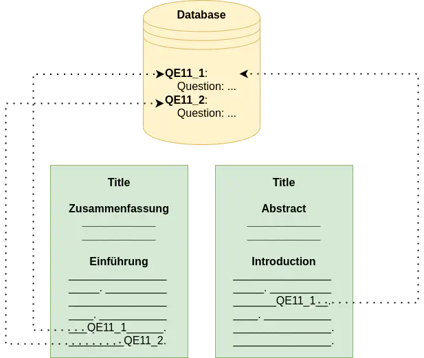 Overview of linking in-text survey variable mentions to a database.
This article demonstrates how to train models for Survey Variable Identification. Currently, the SV-Ident 2022 Shared Task is on-going. Prediction results on the test dataset can be submitted from July 15th until July 25th! Register here to participate!
Introduction
In Social Science research, data collected through survey interviews are typically used to analyze and measure different phenomenon. For example, to study the legitimacy of the European Union, the concept of European identity could used and operationalized (i.e., measurable terms for a concept could be defined). To measure the concept, questions and answers from relevant surveys could then be aggregated. Throughout this article, questions and concepts are both considered survey variables (or just variables). For example, questions on media use and perceived relevance of the sources for news on the EU (e.g., QE11_1/2/3/4) could be combined to measure the amount of contact with European issues. Although, the authors1 acknowledge the limitations of using these variables to measure these defined concepts.
The concepts used and how they are measured in a specific research paper (i.e., which survey variables or other data were used) are typically reported without explicit links. In other words, if a research paper uses the survey variable QE11_1, it may not explictly use a unique identifier to link the research paper to a database of survey variables2 (the example below shows sentences mentioning variables QE11_1/2/3).
“The perceived bias was operationalized by three items. The respondents were asked, “Do you think that the [national] television present(s) the EU too positively, objectively, or too negatively?” The same question was repeated regarding the radio and the press.” - Ejaz et al. (2017)1
Instead, variable metadata (e.g., the question text) is typically mentioned3 once for defining concepts and later implicitly referenced. This is problematic as it often requires social scientists to manually read entire research papers to find, compare, and reproduce results. To alleviate this issue, automatic methods could be used to link in-text variable mentions to external databases of variables. This type of linking could not only be useful on the document-level, but also on the sentence-level, which could allow easier analyses of survey variable usage. To this end, recent advances in Natural Language Processing (NLP) can be used to tackle this problem. The remainder of this article will explain how to train baseline statistical and neural network models for (1) detecting sentences that mention variables and (2) disambiguating the exact variables being mentioned from a list of possible variables.
Data
In Machine Learning (ML), labeled data4 is often required to train models. High-quality labeled data is usually costly and difficult to produce, given that human annotators are required. For the scientific domain, labeled data is even more difficult to produce, as annotators often also need to be “experts” in a scientific discipline.
For NLP in the Social Science, datasets are scarce. However, Zielinski and Mutschke56 released a small dataset (consisting of close to 1,200 sentences) labeled with variable mentions. They split the task of Survey Variable Identification into two sub-tasks: Variable Detection and Variable Disambiguation. They also showed promising initial results.
Recently, in an attempt to extend their work, the Shared Task on Survey Variable Identification has been proposed with the two sub-tasks mentioned above and a larger annotated dataset. The data consist of 4,248 sentences from English and German Social Science publications. The remainder of this article will use this data to train and evaluate different models.
| Sentences w/ variables | Sentences w/o variables | |
|---|---|---|
| English | 859 | 1,232 |
| German | 985 | 1,172 |
| Total | 1,844 | 2,404 |
The data, divided into training and validation sets, can easily be loaded using HuggingFace Datasets (as seen in the image below) or by downloading the data from the GitHub repository.
from datasets import load_dataset

dataset = load_dataset("vadis/sv-ident")
The dataset comes with a number of different fields:
sentence:       Textual instance, which may contain a variable mention.
is_variable:    Label, whether the textual instance contains a variable mention (1) or not (0). This column can be used for Task 1 (Variable Detection).
variable:       Variables (separated by a comma ";") that are mentioned in the textual instance. This column can be used for Task 2 (Variable Disambiguation). Variables with the "unk" tag could not be mapped to a unique variable.
research_data:  Research data IDs (separated by a ";") that are relevant for each instance (and in general for each "doc_id").
doc_id:         ID of the source document. Each document is written in one language (either English or German).
uuid:           Unique ID of the instance in uuid4 format.
As can be seen, sentence contains the text, is_variable contains a binary label (0 or 1) for whether the example mentions a variable or not, and variable contains a list of unique variable IDs that are mentioned in the example. Depending on the task, different fields may be necessary and/or helpful for solving it. An example instance is shown below:
{
  'sentence': 'Additionally, the available indicators of media use combined with the perceived relevance of these sources for news on the EU might be considered of questionable appropriateness in measuring the amount of contact with European issues.',
  'is_variable': 1,
  'variable': ['exploredata-ZA5876_Varqd3_2', 'exploredata-ZA5876_Varqe11_1', exploredata-ZA5876_Varqe11_2', 'exploredata-ZA5876_Varqd3_3', 'exploredata-ZA5876_Varqd3_1',
 'exploredata-ZA5876_Varqe11_3'],
  'research_data': ['ZA5876'],
  'doc_id': '55534',
  'uuid': '5ae61f97-0240-4b3d-9671-0f0d22757d3b',
  'lang': 'en'
}
Variable Detection
The task of Variable Detection can be formulated as binary sentence classification: given a sentence, classify whether it contains a variable or not. In the following, I will demonstrate how to train two different models: logistic regression and BERT.7
Logistic Regression
The logistic regression model is a simple linear model that can be used in binary classification tasks. Before training the model, the data needs to be converted from discrete text into a numerical representation. To do this, we can simply create a vocabulary of words in all examples (using sklearn’s CountVectorizer), and then count the words in each example (using the transform function).
from sklearn.feature_extraction.text import CountVectorizer

vectorizer = CountVectorizer()
X_train = vectorizer.fit_transform(dataset["train"]["tokens"]).toarray()
X_val = vectorizer.transform(dataset["validation"]["tokens"]).toarray()
The counts, in addition to the labels, can then be used as input features for the model. The model can then be trained in under a minute.
from sklearn.linear_model import LogisticRegression
import numpy as np
np.random.seed(42)  # set seed for reproducibility

y_train = np.array(train_dataset['is_variable'])

classifier = LogisticRegression()
classifier.fit(X_train, y_train)
The trained classifier can then be used to make predictions on unseen examples from the validation set.
y_val = np.array(test_dataset['is_variable'])
y_pred = classifier.predict(X_test)
Using F1-macro, we can then evaluate the performance of the model.
from sklearn.metrics import f1_score

print(f1_score(y_val, y_pred, average="macro"))
>>
0.7210459976417424
As can be seen, the model was able to achieve an F1-macro performance of 72.1%. The code to reproduce the results can also be found and executed in this Colab notebook. A more detailed notebook can be found here.
BERT
A more complex model is BERT,7 which is a bi-directional transformer model that was pre-trained on a large text corpus.8 BERT is used to transform text into dense vectors (i.e., features) that “carry” semantic meaning, and it can be fine-tuned on a specific task. For many tasks, this type of training, called transfer learning, outperforms training from scratch (as was done in the logistic regression example).
In this article, the a distilled version of BERT (DistilBERT) will be used, which is smaller in size and trains faster, however, has lower performance than the full BERT model. First, the tokenizer and model need to be loaded. In order to make this model training setting more comparable to the previous one, the sentences will be lowercased. Due to memory constraints, the input to BERT is typically not longer than a set threshold. Here, the maximum length will be set to 128. A number of additional hyperparameters need to be set, which will not be discussed in detail in this article.
from transformers import AutoConfig, AutoModelForSequenceClassification, AutoTokenizer
import numpy as np
import torch
import random

seed = 42
random.seed(seed)
np.random.seed(seed)
torch.manual_seed(seed)
if torch.cuda.is_available():
    torch.cuda.manual_seed_all(seed)

lowercase = True
max_len = 128
model_name = "distilbert-base-uncased"
tokenizer = AutoTokenizer.from_pretrained(model_name, use_fast=True)
tokenizer.do_lower_case = lowercase

model_config = AutoConfig.from_pretrained(model_name)
model_config.num_labels = 2

model = AutoModelForSequenceClassification.from_pretrained(model_name, config=model_config)
The data then needs to tokenized using the loaded tokenizer from the model, which has a specific vocabulary of sub-word units. Here, a custom Dataset class is used to do the transformation.
from datasets import load_dataset

class Dataset:
    def __init__(self, dataset, lowercase=False, batch_size=16, max_len=64):
        self.dataset = dataset
        self.lowercase = lowercase
        self.batch_size = batch_size
        self.max_len = max_len

    def _encode(self, example):
        return self.tokenizer(
            example["sentence"],
            truncation=True,
            max_length=self.max_len,
            padding="max_length",
        )

    def format(self, dataset):
        dataset = dataset.map(self._encode, batched=True)
        try:
            dataset.set_format(
                type="torch",
                columns=["input_ids", "token_type_ids", "attention_mask", "label"],
            )
        except:
            try:
                dataset.set_format(
                type="torch",
                columns=["input_ids", "attention_mask", "label"],
            )
            except:
                raise Exception("Unable to set columns.")
        return dataset

    def format_data(self, tokenizer, batch_size=None):
        self.tokenizer = tokenizer
        if batch_size:
            self.batch_size = batch_size

        self.train_dataset = self.format(self.dataset["train"])
        self.val_dataset = self.format(self.dataset["val"])


orig_dataset = load_dataset("vadis/sv-ident")
orig_dataset = orig_dataset.rename_column("is_variable", "label")

dataset = Dataset({"train": orig_dataset["train"], "val": orig_dataset["validation"]})
dataset.format_data(tokenizer)
Using HuggingFace’s Trainer class is a straightforward method of training models. It takes as input a numer of hyperparameters, some of which will be set.
epochs = 5
training_args = TrainingArguments(
    output_dir=".",
    num_train_epochs=epochs,
    per_device_train_batch_size=16,
    per_device_eval_batch_size=16 * 4,
    evaluation_strategy="steps",
    eval_steps=100,
    seed=seed,
)

trainer = Trainer(
    model=model,
    args=training_args,
    compute_metrics=compute_metrics,
    train_dataset=dataset.train_dataset,
    eval_dataset=dataset.val_dataset,
    tokenizer=tokenizer,
)
The model can then be easily trained and evaluated.
trainer.train()
res = trainer.evaluate()

print(res["eval_f1-score"])
>>
0.7725211139845287
The DistilBERT model outperforms the logistic regression model by about 5%. Using the full BERT model or more recent models can further improve performance. The code to reproduce the results can also be found and executed in this Colab notebook. A more detailed notebook can be found here.
For Variable Detection, this article trained models for both English and German data jointly. However, certain models perform better for one language and other for another. For example, BERT was only pre-trained on English texts, while German-BERT9 was pre-trained on German texts.
Variable Disambiguation
The second and more challenging task for identifying variable mentions is Variable Disambiguation. It deals with identifying which variable(s) from a candidate set of hundreds or thousands of variables is being referenced for a given sentence containing a variable mention. A simple formulation for the task is retrieval: given a large set of candidate variables, retrieve the top k most likely relevant variables. To further simplify the task, rather than requiring the full architecture of an Information Retrieval system, this article will only demonstrate how to run pair-wise vector similarity computations. More specifically, each sentence containing a variable mention will be compared to the variable metadata for the candidate variables. The assumption here is that the more similar a variable mention and the metadata are, the more likely the sentence is in fact referencing this variable. In other words, the similarity scores will as proxies. The most similar k variables will then be considered as predictions for a given example.
Cosine Similarity using Bag-of-Words
Different from the previous examples, in addition to loaded the dataset, the variable metadata also needs to be downloaded and loaded. The variable metadata is available here and can be downloaded manually or programmatically.
import gdown

gdown.download("https://drive.google.com/uc?id=18slgACOcE8-_xIDX09GrdpFSqRRcBiON", "./variables_metadata.json")
In this article, the variable metadata is simply “flattened” (i.e., all metadata values for a variable as combined together). The data can then be converted into vector format, similar to the logistic regression example.
import json
from datasets import load_dataset
from sklearn.feature_extraction.text import CountVectorizer

def combine_metadata(metadata):
    variables = {}
    for rd_id,all_variable in metadata.items():
        combined_variables = {}
        for v_id,variable_metadata in all_variable.items():
            flat_metadata = [m.replace(";", " ") if isinstance(m, str) else " ".join(m).replace(";", " ") for m in list(variable_metadata.values())]
            combined_variables[v_id] = " ".join(flat_metadata)
        variables[rd_id] = combined_variables
    return variables

with open("./variables_metadata.json", "r") as fp:
    metadata = json.load(fp)
flat_metadata = combine_metadata(metadata)

dataset = load_dataset("vadis/sv-ident")

vectorizer = CountVectorizer()
X_train = vectorizer.fit_transform(valid_train_dataset["sentence"]).toarray()
X_val = vectorizer.transform(valid_val_dataset["sentence"]).toarray()
The research data IDs can be used to generate the full list of possible candidate variables for a given example. Because only those instances are relevant, which actually contain variables, the dataset can be filtered down heuristically. The assumption here is that sentences without variable mentions are filtered using Variable Detection. Then, using brute-force, all sentences can be compared to all possible variables, given that the set of possible variables is usually smaller than 5,000 for the datasets used here.
from sklearn.metrics.pairwise import cosine_similarity
from tqdm.notebook import tqdm

top_k = 10

qrels = {}
results = {}

for example,X_vec in tqdm(zip(valid_val_dataset, X_val), total=len(valid_val_dataset)):
    uuid = example["uuid"]
    rd_ids = example["research_data"]
    variables = example["variable"]

    qrels[uuid] = {v:1 for v in variables}

    relevant_variables = {}
    for rd_id in rd_ids:
        rel_vars = flat_metadata[rd_id]
        for k,v in rel_vars.items():
            assert k not in relevant_variables
            relevant_variables[k] = vectorizer.transform([v]).toarray()

    local_res = {}
    for k,v in relevant_variables.items():
        local_res[k] = cosine_similarity([X_vec], v)[0][0]

    slocal_res = {k: v for k, v in sorted(local_res.items(), key=lambda item: item[1], reverse=True)}
    top_k_res = {}
    for k,v in slocal_res.items():
        top_k_res[k] = v

    results[uuid] = top_k_res
The format used for evaluating the results (which is the same format required for submitting results to the Shared Task) contains a mapping between the document IDs and the relevant variables. In the gold data, each relevant variable contains is given a relevance rating of 1.
{
  'd9ae3784-0668-4896-a376-51bdcc68accc': {
    'exploredata-ZA5876_Varqd2_1': 1,
    'exploredata-ZA5876_Varqd3_1': 1,
    'exploredata-ZA5876_Varqd3_2': 1,
    'exploredata-ZA5876_Varqd3_3': 1
  },
  ...
}
The predictions file has the same format, but instead, all variables are given a relevance score equal to their cosime similarity between the variable and the sentence vectors.
{
  'e4467c6e-f312-4736-9d5a-dd6637e37ae1': {
    'exploredata-ZA4600_VarV148': 0.10390312844148933,
    'exploredata-ZA4600_VarV381': 0.1012066801612248,
    'exploredata-ZA4600_VarV384': 0.10029761970569848,
    'exploredata-ZA4600_VarV84': 0.10046604779771835,
    'exploredata-ZA4600_VarV85': 0.10051636888667267,
    'exploredata-ZA4600_VarV86': 0.10036563193274914,
    'exploredata-ZA4600_VarV87': 0.09981867618808633,
    'exploredata-ZA4600_VarV88': 0.10107493851032807,
    'exploredata-ZA4600_VarV89': 0.1008198915771804,
    'exploredata-ZA4600_VarV91': 0.10133193088678279,
    'exploredata-ZA4600_VarV92': 0.10138356499504404,
    ...
  },
  ...
}
Finally, the gold (here qrels) and results can be evaluated using different metrics. In line with the evaluation metrics for Task 2 in the Shared Task, (Mean) Average Precision with a cutoff of 10 is used (MAP@10). This measure is assumed to be realistic for the task, as it does not require knowledge about the number of relevant variables and it does not directly take the order of the predicted variables into account.10
from ranx import evaluate

print(evaluate(qrels, results, "map@10"))
>>
0.034160486395973286
Using the proposed methods does not seem to not work well, given that a MAP@10 score of 3.4% is low. The code to reproduce the results can also be found and executed in this Colab notebook.
Sentence-Transformers
Sentence representations have recently shown superior performance in sentence-level tasks, which makes them promising for Survey Variable Identification. This article will demonstrate how to use pre-trained models in a zero-shot setting (i.e., without training the model) and show that they outperform the bag-of-words baseline presented above.
The data again needs to be loaded. This time, however, the data takes a column-wise format and sentences without research data links and unk variables are removed.11
import gdown
import json

gdown.download("https://drive.google.com/uc?id=18slgACOcE8-_xIDX09GrdpFSqRRcBiON", "./variables_metadata.json")
with open("./variables_metadata.json", "r") as fp:
    metadata = json.load(fp)

def combine_metadata(metadata):
    variables = {}
    for rd_id,all_variable in metadata.items():
        combined_variables = {}
        for v_id,variable_metadata in all_variable.items():
            flat_metadata = [m.replace(";", " ") if isinstance(m, str) else " ".join(m).replace(";", " ") for m in list(variable_metadata.values())]
            combined_variables[v_id] = " ".join(flat_metadata)
        variables[rd_id] = combined_variables
    return variables

flat_metadata = combine_metadata(metadata)

def drop_unk_variables(df):
    new_rows = []
    for i in range(df.shape[0]):
        row = copy.deepcopy(df.iloc[i])
        variables = row["variable"].split(";") if ";" in row["variable"] else row["variable"]
        vrds = ";".join([v for v in variables if v != "unk"])
        if vrds:
            row["variables"] = vrds
            new_rows.append(row)
    return pd.DataFrame(new_rows)

dataset = load_dataset("vadis/sv-ident")
val_df = pd.DataFrame(dataset)
val_df['research_data'] = val_df['research_data'].apply(lambda x: ";".join(sorted(x))).tolist()
# drop rows w/o research data
val_df = val_df[val_df["research_data"].notna()]
# only evaluate on valid rows
val_df = drop_unk_variables(val_df)
Using the the beir benchmark framework, many different pre-trained sentence-representations can be loaded into a retrieval pipeline. In this article, a single multilingual model will be used to evaluate both English and German sentences, namely paraphrase-multilingual-MiniLM-L12-v2. Similar to the previous example, cosine similarity is the measure used for comparing pairs of vectors.
model_path = "paraphrase-multilingual-MiniLM-L12-v2"

model = DRES(models.SentenceBERT(model_path), batch_size=16)
retriever = EvaluateRetrieval(model, score_function="cos_sim", k_values=[10])
Now, the model can be run to retrieve results on the validation set. The data is first converted into a specific format. The details of the format are not important, but they correspond to the implementation of the retrieval models in beir.12 Then, the results are aggregated over grouped research data IDs. Recall that each document - as a result, each sentence - is linked to a set of research data IDs. These make up the set of possible variables. As such, for each query, only a subset of the variables need to be loaded. In order to speed up this process, queries (i.e., sentences) with the same set of research data IDs are grouped together and evaluated joinly.
# Note: see the colab notebook for the full implementation of the functions and classes

all_results = {}
all_qrels = {}

for name, group in tqdm(val_df.groupby("research_data")):
    ivariables, mapping = get_instance_variables(group, flat_metadata)

    queries = get_queries(group)
    corpus = get_corpus(group, ivariables, mapping)
    qrels = get_qrels(group, mapping)

    data_dir = os.path.join(".", "temp", "beir", name)
    save_files(queries, corpus, qrels, data_dir)

    corpus, queries, qrels = GenericDataLoader(data_folder=data_dir).load(split="all")

    results = retriever.retrieve(corpus, queries, return_sorted=True)

    for k,v in qrels.items():
        assert k not in all_qrels
        all_qrels[k] = v
    for k,v in results.items():
        assert k not in all_results
        all_results[k] = v
Finally, the retireved results can be evaluated.
from ranx import evaluate

scores = evaluate(all_qrels, all_results, ["map@10"])
print(scores)
>>
0.12809949092608866
Sentence representations give a slight boost in performance, which reaches 16.1% for English sentences. For German, performance reaches %. The code to reproduce the results can also be found and executed in this Colab notebook.
For Variable Disambiguation, this article used multilingual models for evaluating both English and German data. However, certain models may perform better for certain languages, given that pair-wise sentence training data is more abundant for English than for German.
Conclusion
This article showed how to implement simple statistical and neural baselines for Variable Detection and Disambiguation. Given that the task for Survey Variable Identification is new, exploration of different architectures and methods is needed. In addition, because the task is application-oriented, research on the task can have real and immediate impact. The SV-Ident 2022 Shared Task is a collective research challenge with the goal of understanding how different approaches to Survey Variable Identification perform in a multlilingual setting. The training and validation data used in this article originate from the data release for SV-Ident 2022. Test data, for which participants will submit prediction results, will be released on July 15th, 2022. Results can be submitted until July 25th. For more information, visit the homepage of SV-Ident 2022.
References
-
Ejaz, W., Bräuer, M., & Wolling, J. (2017). Subjective Evaluation of Media Content as a Moderator of Media Effects on European Identity: Mere Exposure and the Hostile Media Phenomenon. Media and Communication, 5(2), 41-52. doi:https://doi.org/10.17645/mac.v5i2.885 ↩︎ ↩︎
-
For example, GESIS has a database of over 500k survey variables. ↩︎
-
Variable metadata can be mentioned in different ways. For example, exact quotations or paraphases of multiple variables could be used. ↩︎
-
In Social Science, this can be called “coded.” ↩︎
-
Andrea Zielinski and Peter Mutschke. 2017. Mining Social Science Publications for Survey Variables. In Proceedings of the Second Workshop on NLP and Computational Social Science, pages 47–52, Vancouver, Canada. Association for Computational Linguistics. ↩︎
-
Andrea Zielinski and Peter Mutschke. 2018. Towards a Gold Standard Corpus for Variable Detection and Linking in Social Science Publications. In Proceedings of the Eleventh International Conference on Language Resources and Evaluation (LREC 2018), Miyazaki, Japan. European Language Resources Association (ELRA). ↩︎
-
Jacob Devlin, Ming-Wei Chang, Kenton Lee, and Kristina Toutanova. 2019. BERT: Pre-training of Deep Bidirectional Transformers for Language Understanding. In Proceedings of the 2019 Conference of the North American Chapter of the Association for Computational Linguistics: Human Language Technologies, Volume 1 (Long and Short Papers), pages 4171–4186, Minneapolis, Minnesota. Association for Computational Linguistics. ↩︎ ↩︎
-
The corpus included 2,500M words from Wikipedia pages and 800M words from books. ↩︎
-
Branden Chan, Stefan Schweter, and Timo Möller. 2020. German’s Next Language Model. In Proceedings of the 28th International Conference on Computational Linguistics, pages 6788–6796, Barcelona, Spain (Online). International Committee on Computational Linguistics. ↩︎
-
The precision at a recall level of 5 with 2 correct variables, is 40% regardless of whether the predictions are in the first or last two slots. However, because the average over different recall levels is computed, having correct predictions at a lower recall level increases the score (e.g., 1/1+2/2 > 0/1+2/2). ↩︎
-
Annotators marked sentences with the
unkvariable tag in cases where they were unable to find the correct variable, but were confident that a variable was mentioned. Such examples are kept in the dataset, as the sentences can still be used for Variable Detection. ↩︎ -
A number of functions as well as the
GenericDataLoaderandSentenceBERTclasses were overritten and excluded in the code snippets due to space constraints. See the full implementation in the Colab notebook. ↩︎
Tornike Tsereteli
/tʰɔrnikʼɛ tsʼɛrɛtʰɛli/
I am a PhD candidate in Computational Linguistics candidate at the University of Mannheim. I work on Natural Language Processing and Machine Learning.